How to (Efficiently) Process Change Data Feed in Databricks Delta

Recently, the AUTO CDC pipeline command added a new option: WITH (readChangeFeed=true), which enables out-of-the-box processing of Change Data Feed from Delta using AUTO CDC. It's also now possible to orchestrate the AUTO CDC pipeline from a SQL warehouse.

"AUTO CDC is the easy button for incremental data processing. Instead of managing complex MERGE INTO logic, teams can declaratively build SCD Type 1 and Type 2 models and operationalize CDC in just a few lines of SQL — turning change data feeds into reliable downstream tables with minimal effort."
— Shanelle Roman, Product Manager, Databricks

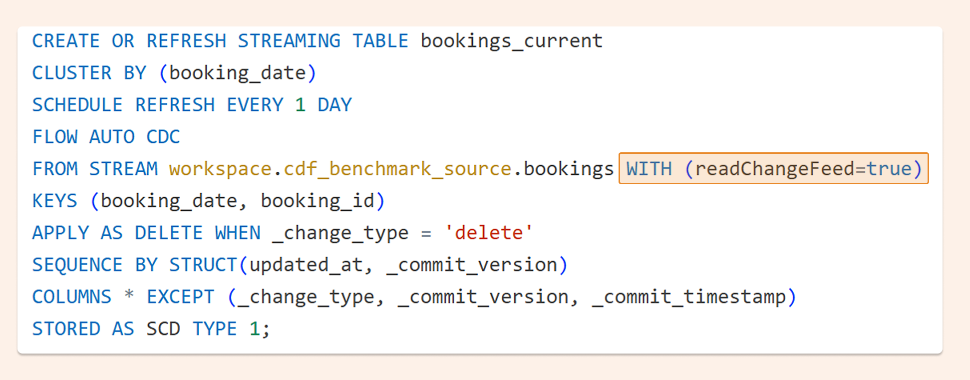
Below is the new syntax for orchestrating a pipeline from a SQL warehouse:

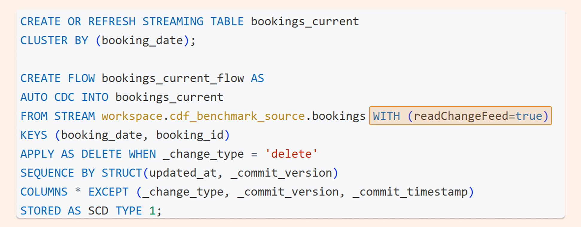
And the syntax used in Spark Declarative Pipelines:

Change Data Feed - what is it?

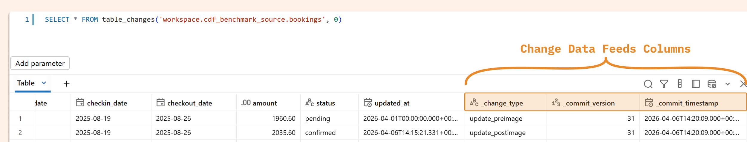
In Delta, you can enable Change Data Feed on a table (TBLPROPERTIES (delta.enableChangeDataFeed = true)). Once enabled, every row-level change is tracked — INSERT, UPDATE, and DELETE.

When consuming CDF, you typically want to build another table from it. That table can either keep only the latest version of each row (SCD Type 1) or maintain a full history (SCD Type 2). In this test, I used SCD Type 1 for simple ingestion from CDF.

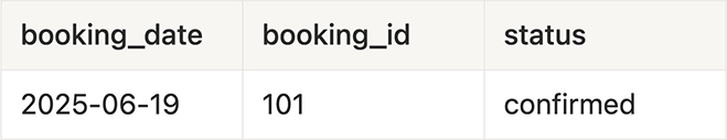
For example, given these source rows:

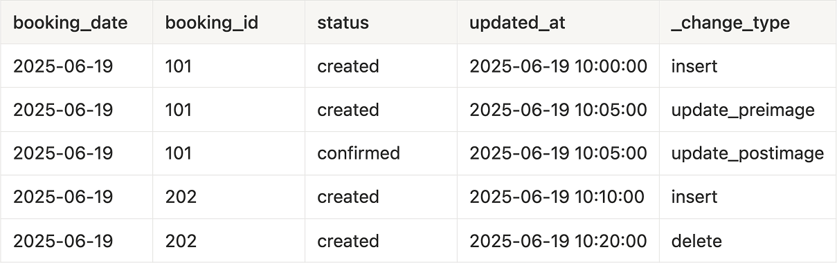
With CSD type 1, you will get just that one record:

The source table received 25 million operations across five test runs, growing the target to 72 million records. The question was simple: which approach processes that workload most cheaply?

CDF Ingestion Test: 3 Approaches

The test compared three ways to process Change Data Feed on Databricks, each run in both standard and performance mode where applicable.

AUTO CDC got me curious about a practical question: if it's now one of the easiest ways to process CDF, is it also the cheapest?

To find out, I compared three approaches:

• AUTO CDC pipeline (in standard and performance mode)

• Spark Structured Streaming (in standard and performance mode)

• SQL warehouse with table_changes()

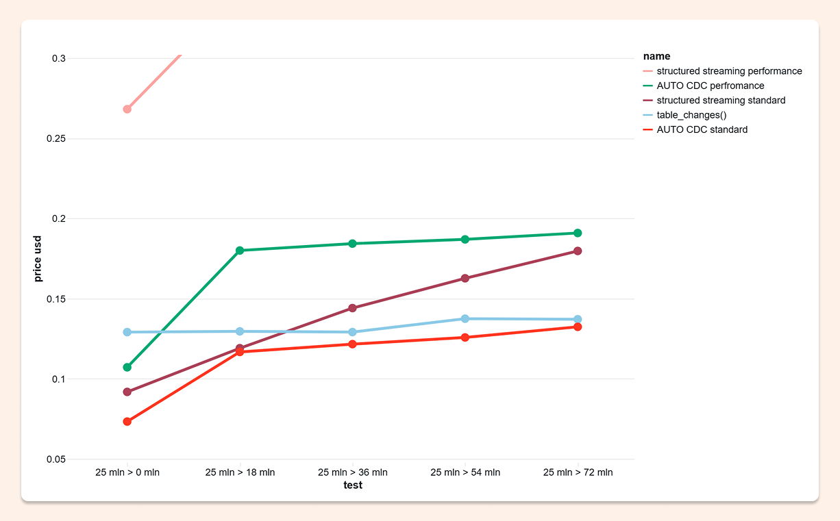
I performed 25 million operations (INSERT, UPDATE, DELETE) on the source dataset and ran each test five times. The target table started with 0 rows and grew to 72 million records across runs. Afterward, I built the charts below using job tags and usage policy tags.

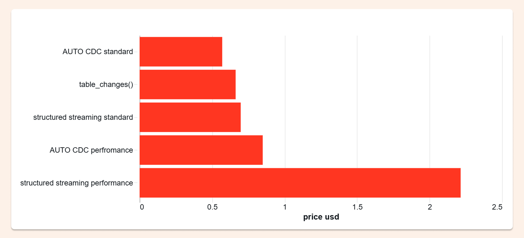
I was genuinely surprised: AUTO CDC won. It was the cheapest option in every run, even as the dataset kept growing.

That said, each approach has its own strengths. And honestly, all three came in at very reasonable prices — moments like this remind you why Databricks is such a compelling platform. So let's start with the winner.

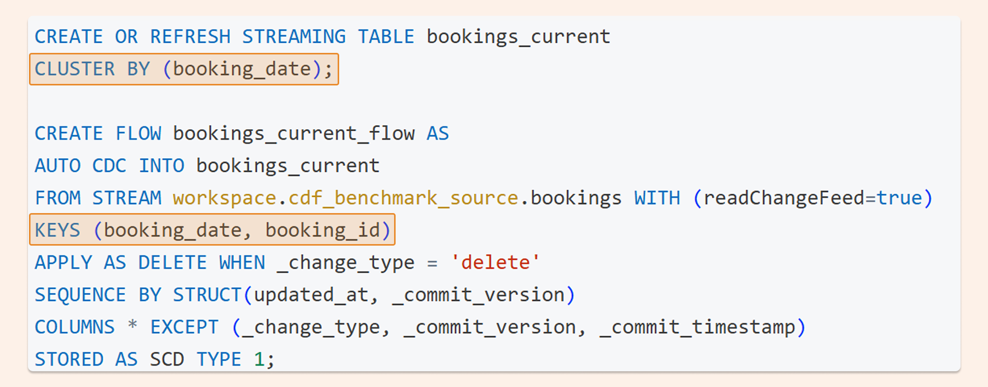
1. AUTO CDC Pipeline

AUTO CDC is part of Databricks' declarative pipelines family. Behind the scenes, Databricks has been steadily improving the price-performance of declarative pipelines through backend work — including Enzyme, Photon, and autoscaling. That makes AUTO CDC interesting not just from a developer productivity standpoint, but from a cost standpoint too.

CREATE OR REFRESH STREAMING TABLE bookings_current
CLUSTER BY (booking_date);

CREATE FLOW bookings_current_flow AS
AUTO CDC INTO bookings_current
FROM STREAM workspace.cdf_benchmark_source.bookings WITH (readChangeFeed=true)
KEYS (booking_date, booking_id)
APPLY AS DELETE WHEN _change_type = 'delete'
SEQUENCE BY STRUCT(updated_at, _commit_version)
COLUMNS * EXCEPT (_change_type, _commit_version, _commit_timestamp)
STORED AS SCD TYPE 1;

Pros:

• Fastest option in my test

• An easy, out-of-the-box way to process CDF with clean SQL syntax

• Handles edge cases that are easy to miss in custom logic — for example, late-arriving data

Cons:

• In some scenarios, the syntax can feel limiting

2. table_changes() on SQL Warehouse

table_changes() is a solid option when you want to stay close to SQL.

SET VAR latest_per_key_sql = "
CREATE OR REPLACE TEMP VIEW staged AS
WITH changes AS (
  SELECT *
  FROM table_changes('" || :source_table || "', " || :start_version || ", " || :end_version || ")
  WHERE _change_type <> 'update_preimage'
)
SELECT *
FROM (
  SELECT
    *,
    row_number() OVER (
      PARTITION BY booking_id, booking_date
      ORDER BY updated_at DESC, _commit_version DESC, _commit_timestamp DESC
    ) AS rn
  FROM changes
)
WHERE rn = 1;
";

EXECUTE IMMEDIATE latest_per_key_sql;

-- MERGE command ON key booking_date and booking_id

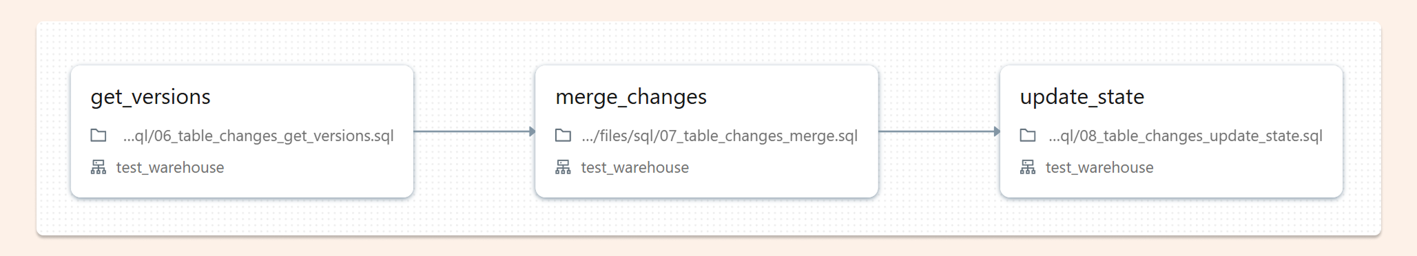
Lakeflow orchestration for managing state:

3. Structured Streaming

Structured Streaming is the most flexible of the three options.

Pros:

• Best choice when you need custom logic

• Works well when you don't want to process every change type the same way — for example, if you only want to handle deletes. foreachBatch can support almost any scenario, and in simpler cases, it can be very efficient

Cons:

• Handling every scenario can make the code complex. In those cases, AUTO CDC is usually the easier path

def upsert_cdf(microbatch_df, batch_id):
    # sort and MERGE command ON key booking_date and booking_id

(
    spark.readStream
    .option("readChangeFeed", "true")
    .option("startingVersion", starting_version)
    .table(source_table)
    .writeStream
    .option("checkpointLocation", checkpoint_path)
    .trigger(availableNow=True)
    .foreachBatch(upsert_cdf)
    .start()
    .awaitTermination()
)

The Benchmark Results

AUTO CDC was the cheapest option in every single run, and maintained that advantage as the dataset grew. That last part matters: this wasn't a small-data result. The cost advantage held at scale.

That said, this isn't a clean knockout. All three approaches produced competitive numbers, and each has a legitimate use case:

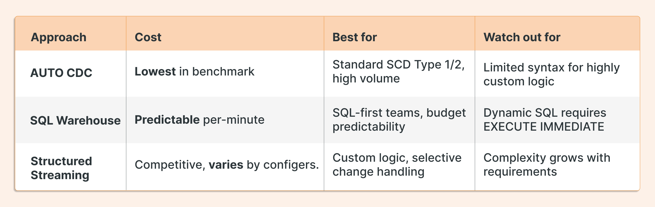
The Partition Trick That Makes All Three Faster

Regardless of which approach you use, there's one optimization that consistently reduces both scan cost and processing time: use two keys instead of one.

When you process CDF with a single high-cardinality key (like a booking ID), the engine has to scan the entire table to find matching rows. Add a low-cardinality key like a date, cluster the target table by that column, and the engine narrows its search space before it ever looks for the ID.

In practice: instead of scanning 72 million rows to find booking ID 101, the engine goes directly to the June 19 partition and scans a fraction of that. Faster processing, lower cost, across all three approaches.

What to Do Next

If your team is processing Change Data Feed today with custom MERGE logic, it's worth running your own benchmark. The full test code, including dashboards and DABS configuration, is available at: github.com/hubert-dudek/medium/tree/main/topics/202604/cdf_benchmark_bundle