Most data teams can land data in a lakehouse. Far fewer can turn it into something the business actually trusts.
The symptoms are familiar. Two dashboards show different revenue numbers for the same quarter. An analyst asks, "How much did we sell to Enterprise customers last year?" and nobody can say whether that means customers who are Enterprise today or customers who were Enterprise when they bought. A Genie space connects to forty Silver tables and confidently starts answering questions with the wrong joins.
This isn't a storage or compute problem. It is a modeling problem.
In this post, we’ll walk through building a dimensional model, a classic Star Schema, on top of Lakeflow Spark Declarative Pipelines (SDP). We cover the design decisions that matter (grain, dimensions, what lives in each layer) and then the implementation: declarative dependencies, data quality expectations, incremental processing, and Slowly Changing Dimensions Type 1 and Type 2 with AUTO CDC. No orchestration code and no hand-written MERGE statements are involved.
Why Dimensional Modeling Still Matters
Every few years someone declares dimensional modeling dead. Storage is cheap, compute is elastic, and columnar engines can scan wide denormalized tables in seconds, so why bother with facts and dimensions?
The answer is that dimensional modeling was never mainly about performance. It is about meaning.
A Star Schema encodes business semantics directly in the structure of the data:
Fact tables record measurable business events, such as an order line, a payment, or a shipment, at a clearly defined grain.
Dimension tables describe the context of those events: who, what, when, where.
Relationships between them are explicit, simple, and predictable: a fact joins to each dimension through a single key.
That simplicity pays off everywhere downstream. BI tools work best with star schemas. Analysts write shorter, more correct SQL. Metrics like net revenue get defined once, in one place, instead of being recalculated slightly differently in every dashboard.
And a newer consumer cares about this more than any human analyst: AI.
Tools like Databricks Genie translate natural-language questions into SQL. Genie is only as good as the data model it reasons over. Give it a sprawl of loosely related tables with ambiguous columns, and it will guess. Give it a well-documented Star Schema, with one fact table at a known grain, conformed dimensions, and clear descriptions, and the guessing mostly disappears. The same structure that made BI reliable twenty years ago is what makes AI-powered analytics reliable today.
If you want a refresher on the fundamentals, the Kimball Group's dimensional modeling techniques and the Databricks overview of the Medallion Architecture are good starting points. Here we focus on the implementation.
The use case: Sales Analytics
To keep things concrete, we will model a typical Sales Analytics scenario. A retail company has three source feeds landing in cloud storage:
Customers: a CRM change feed (inserts, updates, deletes) that includes the customer's segment and country.
Products: a change feed from the product catalog, including category and brand.
Order lines: an export from the ERP, one record per product per order.
The business wants to answer questions like:
What was net revenue by product category and month?
How much revenue came from each customer segment, measured as the segment the customer belonged to at the time of the sale?
Which channels are growing fastest among customers in Spain?
Let's design for those questions first and write code second.
Data Modeling & Design Decisions
The most expensive mistakes in a dimensional model happen before you write any code. Three decisions shape everything else.
Decision 1: The business process and the grain
The business process is sales. The grain, the precise definition of what a single row in the fact table represents, is:
One row per order line.
Not one row per order, and not one row per customer per day. The grain is the atomic event the source system records, and declaring it explicitly is the single most important modeling decision you will make. It determines which measures are additive, which dimensions can attach to the fact, and how every downstream aggregation behaves.
Choosing the lowest available grain also keeps options open. You can always aggregate order lines into orders or daily totals. You can never disaggregate a daily total back into the products that made it up.
Decision 2: Dimensions and measures
With the grain fixed, the dimensions and measures follow naturally.
Measures (numeric, additive at the order-line grain):
quantity
unit_price
discount_amount
net_amount (quantity * unit_price - discount_amount), defined once in the fact table
Dimensions (the context of each sale):
Customer: who bought. Attributes like segment and country_code change over time, and the business wants to analyze sales as they were, so this is an SCD Type 2 dimension.
Product: what was bought. When a product is recategorized, the business wants all history to reflect the current category, so this is an SCD Type 1 dimension.
Date: when it was bought. A generated calendar dimension with year, quarter, month, weekday, and weekend flags.
Low-cardinality attributes such as channel (web, store, marketplace) stay on the fact as degenerate dimensions, alongside the order_id itself.
Notice that the SCD type is a business decision, not a technical one. "Do we want to see revenue under the segment the customer had then, or the one they have now?" is a business question, and the answer changes the model.
For a deeper look at SCD types 0 through 6 and how to implement them with MERGE INTO, see our earlier post: Managing Data Changes with SCDs in Databricks. Here we take the declarative route.
Decision 3: The Star Schema
The resulting model:
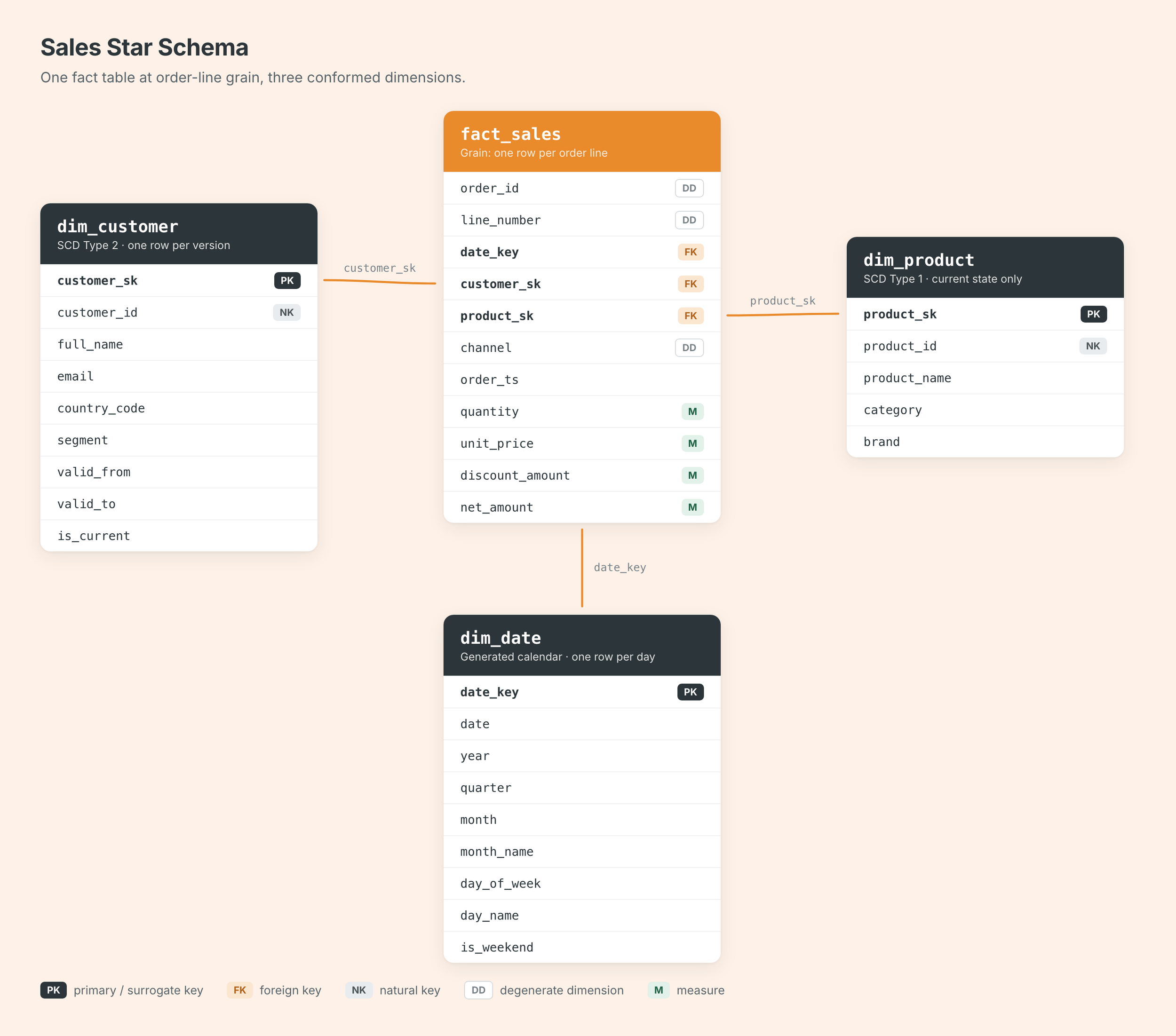
The Sales Star Schema: fact_sales at the order-line grain, surrounded by dim_customer (SCD2), dim_product (SCD1), and dim_date.
Mapping the model to the Medallion Architecture
The Medallion Architecture and dimensional modeling are not competing ideas. Medallion describes how data matures; dimensional modeling describes how mature data is shaped for consumption. They fit together:
Bronze: raw source data. Exactly what the source sent, append-only, with ingestion metadata. No business logic.
Silver: cleansed, standardized, and enriched. Types are cast, values normalized, bad records filtered by expectations, duplicates removed. This is also where change history is resolved: the AUTO CDC targets that hold the full SCD history live here.
Gold: business-ready facts and dimensions. The Star Schema itself, with surrogate keys, friendly column names, validity windows, and business measures. This is the only layer BI tools and Genie should see.
One design choice is worth calling out. We keep the raw AUTO CDC output (with its technical __START_AT / __END_AT columns) in Silver, and publish a clean dimension on top of it in Gold. That keeps the CDC mechanics out of the consumer-facing model and gives us a place to add surrogate keys and business-friendly naming.
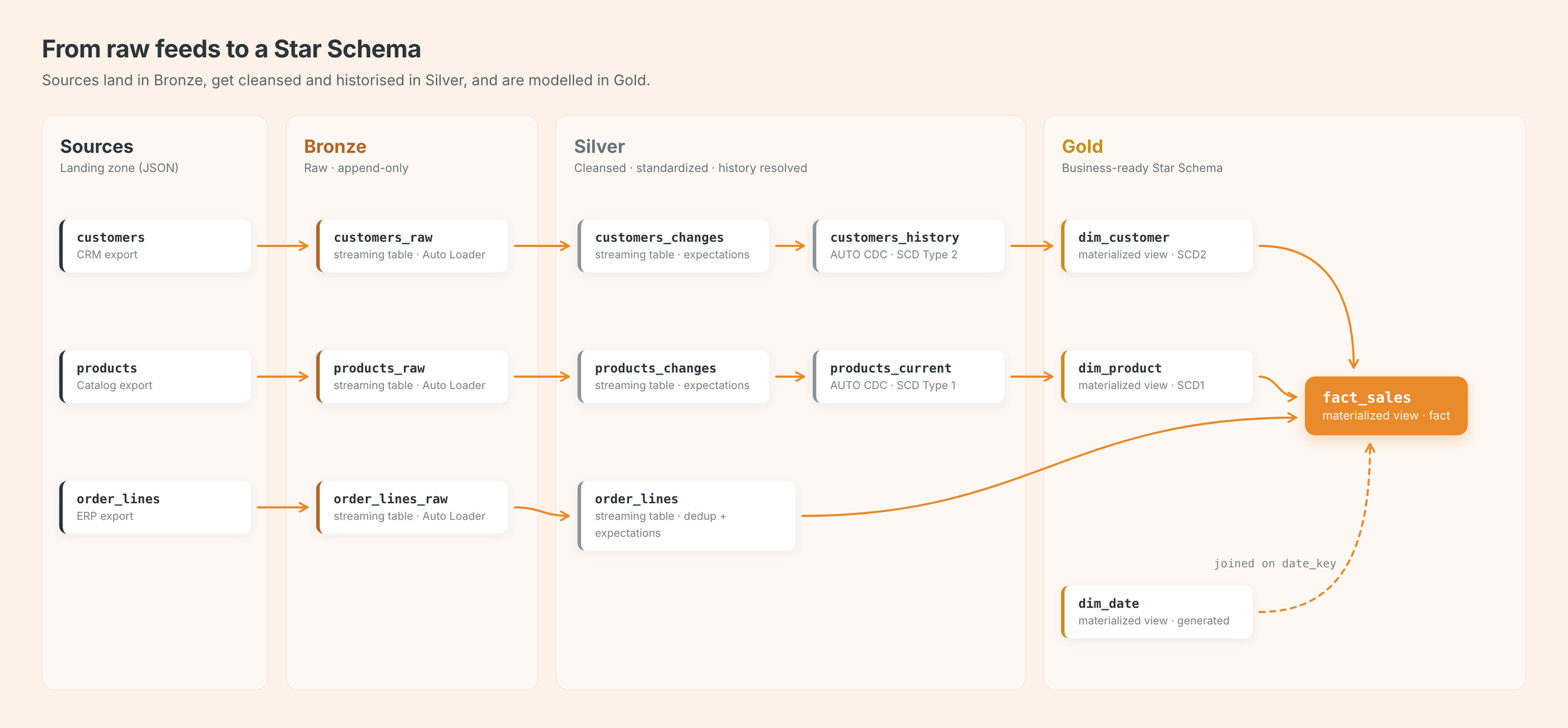
From three raw feeds to a Star Schema: how each table flows through Bronze, Silver, and Gold.
Implementing the Dimensional Model with Spark Declarative Pipelines
Spark Declarative Pipelines (the evolution of Delta Live Tables, now also contributed to Apache Spark) changed the question you answer as a data engineer. With an imperative pipeline, you write how: read this, merge into that, manage this checkpoint, run task B after task A. With SDP, you declare what each dataset is, and the framework works out the rest.
Every table below is just a function that returns a DataFrame. SDP reads those definitions, infers the dependency graph from the tables each function references, and handles execution order, incremental state, retries, and data quality tracking.
We organize the pipeline source code by layer:
src/sales_pipeline/
└── transformations/
    ├── bronze.py
    ├── silver_customers.py
    ├── silver_products.py
    ├── silver_sales.py
    └── gold.py
Bronze: incremental ingestion with Auto Loader
Bronze ingests the three feeds as streaming tables using Auto Loader. Each new file is processed exactly once; SDP manages the checkpoints.
# bronze.py
from pyspark import pipelines as dp
from pyspark.sql import DataFrame
from pyspark.sql import functions as f

LANDING_PATH = spark.conf.get("landing_path")


def ingest(entity: str) -> DataFrame:
    return (
        spark.readStream.format("cloudFiles")
        .option("cloudFiles.format", "json")
        .option("cloudFiles.inferColumnTypes", "true")
        .load(f"{LANDING_PATH}/{entity}")
        .withColumn("_ingested_at", f.current_timestamp())
        .withColumn("_source_file", f.col("_metadata.file_path"))
    )


for entity in ["customers", "products", "order_lines"]:

    @dp.table(
        name=f"bronze.{entity}_raw",
        comment=f"Raw {entity} feed from the landing zone. Append-only, no transformations.",
    )
    def bronze_table(entity: str = entity) -> DataFrame:
        return ingest(entity)
Three tables, one definition. Because pipelines are just Python, metadata-driven patterns like this come for free, and the framework still sees three independent datasets in the graph.
If your sources are Delta tables instead of files, spark.readStream.table() with Change Data Feed gives you the same incremental, CDC-ready input, deletes included.
Silver: cleansing with expectations
Silver is where you enforce data quality. SDP expectations are declarative constraints attached to a dataset, with three possible actions:
@dp.expect: warn. Keep the record and track the violation in the pipeline metrics.
@dp.expect_or_drop: drop. Discard the record and track the violation.
@dp.expect_or_fail: fail. Stop the update, because the data contract is broken.
Choosing the action is, again, a business decision. A malformed email is worth tracking but should not block a sale from being reported. A missing customer key makes the record useless. A currency the model doesn't support means something upstream changed, and someone should check before publishing numbers.
# silver_customers.py
from pyspark import pipelines as dp
from pyspark.sql import DataFrame
from pyspark.sql import functions as f


@dp.table(
    name="silver.customers_changes",
    comment="Cleansed and standardized customer change events from the CRM.",
)
@dp.expect_all_or_drop({
    "valid_customer_id": "customer_id IS NOT NULL",
    "valid_operation": "operation IN ('INSERT', 'UPDATE', 'DELETE')",
    "valid_sequence": "updated_at IS NOT NULL",
})
@dp.expect("valid_email", "email RLIKE '^[^@]+@[^@]+\\\\.[^@]+$'")
def customers_changes() -> DataFrame:
    return (
        spark.readStream.table("bronze.customers_raw")
        .select(
            f.col("customer_id").cast("bigint"),
            f.initcap(f.trim("full_name")).alias("full_name"),
            f.lower(f.trim("email")).alias("email"),
            f.upper(f.trim("country_code")).alias("country_code"),
            f.trim("segment").alias("segment"),
            f.upper("operation").alias("operation"),
            f.to_timestamp("updated_at").alias("updated_at"),
        )
    )
The order lines follow the same pattern, with deduplication. Source exports often re-send the same line after retries or overlapping loads, and the watermark tells Spark how long to remember what it has already seen:
# silver_sales.py
from pyspark import pipelines as dp
from pyspark.sql import DataFrame
from pyspark.sql import functions as f


@dp.table(
    name="silver.order_lines",
    comment="Cleansed, typed, and deduplicated order lines. Grain: one row per order line.",
)
@dp.expect_all_or_drop({
    "valid_keys": "order_id IS NOT NULL AND line_number IS NOT NULL",
    "valid_customer": "customer_id IS NOT NULL",
    "valid_product": "product_id IS NOT NULL",
    "positive_quantity": "quantity > 0",
    "non_negative_price": "unit_price >= 0",
})
@dp.expect_or_fail("supported_currency", "currency = 'USD'")
def order_lines() -> DataFrame:
    return (
        spark.readStream.table("bronze.order_lines_raw")
        .select(
            f.col("order_id").cast("string"),
            f.col("line_number").cast("int"),
            f.col("customer_id").cast("bigint"),
            f.col("product_id").cast("bigint"),
            f.to_timestamp("order_ts").alias("order_ts"),
            f.lower(f.trim("channel")).alias("channel"),
            f.col("quantity").cast("int"),
            f.col("unit_price").cast("decimal(18,2)"),
            f.coalesce(f.col("discount_amount"), f.lit(0)).cast("decimal(18,2)").alias("discount_amount"),
            f.upper("currency").alias("currency"),
        )
        .withWatermark("order_ts", "2 days")
        .dropDuplicatesWithinWatermark(["order_id", "line_number"])
Every expectation appears in the pipeline UI and event log, with pass/fail counts per run. Data quality stops being a separate project and becomes part of the table definition.
Slowly Changing Dimensions with AUTO CDC
This is where SDP saves the most code.
Implementing SCD Type 2 by hand means writing a MERGE that expires the current version of a record, inserts the new version, handles out-of-order events, and deals with deletes, all without breaking when the same batch contains several changes for the same key. Our previous post shows what that looks like. It works, but it is a lot of logic to own.
With AUTO CDC, you declare the target, the key, the ordering column, and the SCD type:
# silver_customers.py (continued)

dp.create_streaming_table(
    name="silver.customers_history",
    comment="Full change history of customers (SCD Type 2), maintained by AUTO CDC.",
)

dp.create_auto_cdc_flow(
    target="silver.customers_history",
    source="silver.customers_changes",
    keys=["customer_id"],
    sequence_by=f.col("updated_at"),
    apply_as_deletes=f.expr("operation = 'DELETE'"),
    except_column_list=["operation"],
    stored_as_scd_type=2,
    # Name or email corrections (and the change timestamp itself) should not create a new version
    track_history_except_column_list=["full_name", "email", "updated_at"],
)
A few things are happening here:
sequence_by orders the events. If an update from Tuesday arrives after one from Wednesday, AUTO CDC still produces the correct history. Out-of-order data is handled for you.
stored_as_scd_type=2 adds __START_AT and __END_AT columns. Each change to a tracked attribute closes the current version and opens a new one; the current version has a null __END_AT.
track_history_except_column_list is a modeling decision written as code. A change in segment or country_code creates a new version, because those attributes affect how sales are analyzed. A typo fix in full_name or a new email simply updates the current row in place. That is a hybrid Type 1/Type 2 behavior with a single parameter. Note that updated_at belongs in this list too: every change event carries a new timestamp, so if it were tracked, any update would open a new version.
apply_as_deletes closes the record when the CRM reports a deletion, preserving its history for past sales.
The product dimension is SCD Type 1. Only the current state matters, so the same API needs just one value changed:
# silver_products.py
from pyspark import pipelines as dp
from pyspark.sql import DataFrame
from pyspark.sql import functions as f


@dp.table(name="silver.products_changes", comment="Cleansed product change events.")
@dp.expect_all_or_drop({
    "valid_product_id": "product_id IS NOT NULL",
    "valid_sequence": "updated_at IS NOT NULL",
})
def products_changes() -> DataFrame:
    return (
        spark.readStream.table("bronze.products_raw")
        .select(
            f.col("product_id").cast("bigint"),
            f.trim("product_name").alias("product_name"),
            f.initcap(f.trim("category")).alias("category"),
            f.initcap(f.trim("brand")).alias("brand"),
            f.upper("operation").alias("operation"),
            f.to_timestamp("updated_at").alias("updated_at"),
        )
    )


dp.create_streaming_table(
    name="silver.products_current",
    comment="Current state of each product (SCD Type 1), maintained by AUTO CDC.",
)

dp.create_auto_cdc_flow(
    target="silver.products_current",
    source="silver.products_changes",
    keys=["product_id"],
    sequence_by=f.col("updated_at"),
    apply_as_deletes=f.expr("operation = 'DELETE'"),
    except_column_list=["operation"],
    stored_as_scd_type=1,
)
Two dimensions, two SCD strategies, and no MERGE statements.
Gold: the Star Schema
Gold is where the Silver datasets become the model the business sees. These are materialized views: their content is fully defined by a query, and SDP keeps them up to date. In serverless pipelines, materialized views refresh incrementally whenever the query allows, so only the affected data is recomputed instead of the whole table.
The customer dimension turns the technical SCD2 output into a consumer-friendly dimension with a surrogate key, readable validity columns, and an is_current flag:
# gold.py
from pyspark import pipelines as dp
from pyspark.sql import DataFrame
from pyspark.sql import functions as f


@dp.materialized_view(
    name="gold.dim_customer",
    comment=(
        "Customer dimension (SCD Type 2). One row per customer version. "
        "Use is_current = true for the latest state of each customer."
    ),
)
def dim_customer() -> DataFrame:
    return (
        spark.read.table("silver.customers_history")
        .select(
            f.xxhash64("customer_id", "__START_AT").alias("customer_sk"),
            "customer_id",
            "full_name",
            "email",
            "country_code",
            "segment",
            f.col("__START_AT").alias("valid_from"),
            f.col("__END_AT").alias("valid_to"),
            f.col("__END_AT").isNull().alias("is_current"),
        )
    )


@dp.materialized_view(
    name="gold.dim_product",
    comment="Product dimension (SCD Type 1). One row per product, current attributes only.",
)
def dim_product() -> DataFrame:
    return (
        spark.read.table("silver.products_current")
        .select(
            f.col("product_id").alias("product_sk"),
            "product_id",
            "product_name",
            "category",
            "brand",
        )
    )
A word on surrogate keys. In an SCD Type 2 dimension, customer_id is no longer unique: every version of a customer shares it. The fact table needs to point to one specific version, and that is the job of customer_sk. With it, every downstream query joins facts and dimensions through a single, simple equality (f.customer_sk = c.customer_sk), and the point-in-time logic lives in one place: the fact table build.
We derive the key with a hash of the natural key and the version start (xxhash64(customer_id, __START_AT)) instead of an auto-generated sequence or identity column. The reason is determinism. Materialized views can be recomputed, and any table can be fully refreshed; a hash guarantees that the same customer version always gets the same key, so facts and dimensions stay consistent without coordinating sequence state between them.
Two details worth knowing. First, product_sk is simply the product_id: dim_product is SCD Type 1, so there is exactly one row per product and the natural key is already unique. We still expose it as product_sk to keep the model uniform, and so that the fact table does not change if the dimension ever evolves to SCD Type 2. Second, xxhash64 produces a 64-bit value, so collisions are possible in theory but negligible at typical dimension volumes. If you need a hard guarantee, sha2 works the same way at the cost of a longer string key.
The date dimension is generated rather than ingested:
@dp.materialized_view(
    name="gold.dim_date",
    comment="Calendar dimension. One row per day. date_key format: yyyyMMdd.",
)
def dim_date() -> DataFrame:
    return (
        spark.sql(
            "SELECT explode(sequence(DATE'2020-01-01', DATE'2030-12-31', INTERVAL 1 DAY)) AS date"
        )
        .select(
            f.date_format("date", "yyyyMMdd").cast("int").alias("date_key"),
            "date",
            f.year("date").alias("year"),
            f.quarter("date").alias("quarter"),
            f.month("date").alias("month"),
            f.date_format("date", "MMMM").alias("month_name"),
            f.dayofweek("date").alias("day_of_week"),
            f.date_format("date", "EEEE").alias("day_name"),
            f.dayofweek("date").isin(1, 7).alias("is_weekend"),
        )
    )
The fact table brings it together. The key detail is the point-in-time join to the SCD2 customer dimension: each order line is matched to the customer version that was valid when the order was placed.
@dp.materialized_view(
    name="gold.fact_sales",
    comment=(
        "Sales fact. Grain: one row per order line. "
        "net_amount = quantity * unit_price - discount_amount. "
        "customer_sk points to the customer version valid at order time."
    ),
)
@dp.expect("customer_version_resolved", "customer_sk IS NOT NULL")
@dp.expect("product_resolved", "product_sk IS NOT NULL")
def fact_sales() -> DataFrame:
    lines = spark.read.table("silver.order_lines").alias("l")
    customers = spark.read.table("gold.dim_customer").alias("c")
    products = spark.read.table("gold.dim_product").alias("p")

    customer_as_of_order = (
        (f.col("l.customer_id") == f.col("c.customer_id"))
        & (f.col("l.order_ts") >= f.col("c.valid_from"))
        & (f.col("c.valid_to").isNull() | (f.col("l.order_ts") < f.col("c.valid_to")))
    )

    return (
        lines
        .join(customers, customer_as_of_order, "left")
        .join(products, f.col("l.product_id") == f.col("p.product_id"), "left")
        .select(
            f.col("l.order_id"),
            f.col("l.line_number"),
            f.date_format("l.order_ts", "yyyyMMdd").cast("int").alias("date_key"),
            f.col("c.customer_sk"),
            f.col("p.product_sk"),
            f.col("l.channel"),
            f.col("l.order_ts"),
            f.col("l.quantity"),
            f.col("l.unit_price"),
            f.col("l.discount_amount"),
            (f.col("l.quantity") * f.col("l.unit_price") - f.col("l.discount_amount"))
            .cast("decimal(18,2)")
            .alias("net_amount"),
        )
    )
The two @dp.expect rules on the fact use warn, not drop. An order line whose customer version cannot be resolved (for example, an order that arrives before the CRM change that created the customer) is still a real sale and should be counted in revenue. The expectation makes the problem visible in the pipeline metrics without silently losing money from the report.
What SDP is doing that you are not
Look at the pipeline graph SDP produces from the code above:
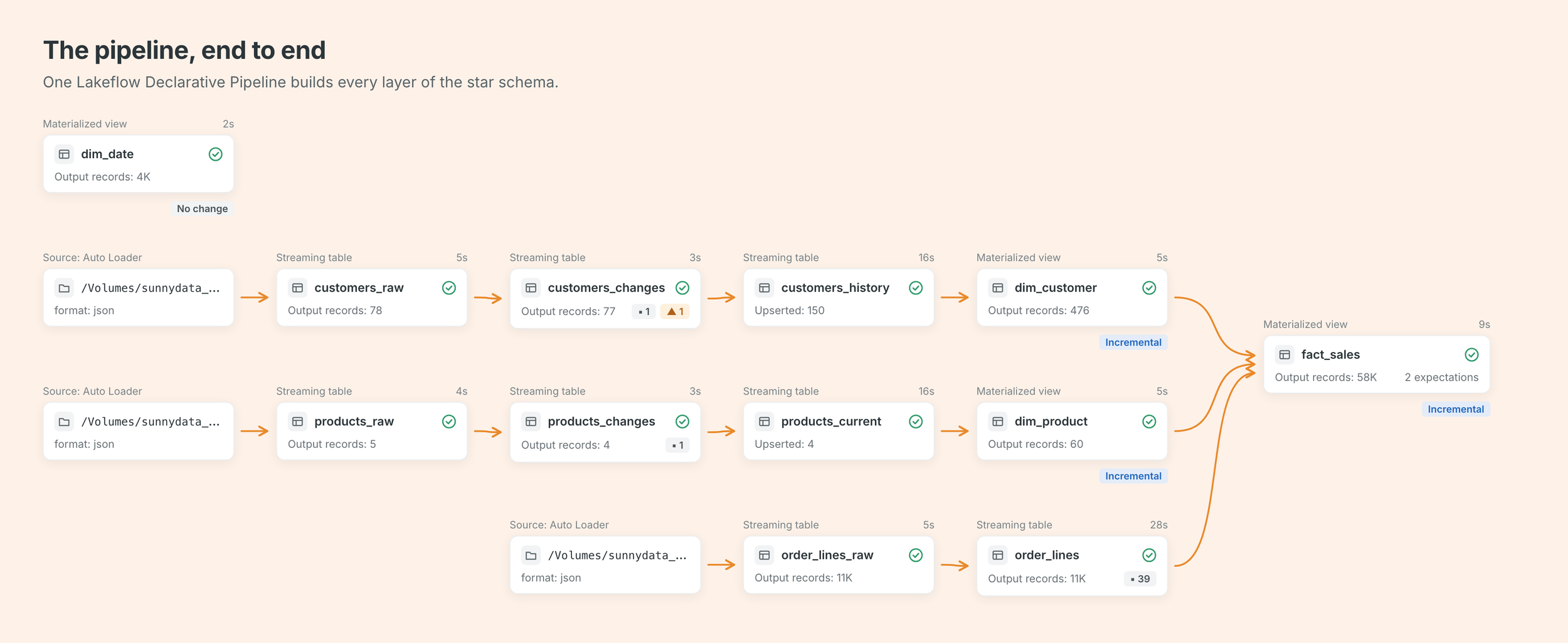
The dependency graph inferred by SDP. No task definitions, no depends_on: every edge comes from a spark.read.table or spark.readStream.table reference.
Nowhere did we write orchestration logic. There are no tasks, no depends_onand no "run Silver after Bronze" step. Here is what the framework handled on its own:
Dependencies. fact_sales reads gold.dim_customer, which reads silver.customers_history, which is fed by silver.customers_changes. SDP infers the full DAG and runs it in the right order, in parallel where it can.
Incremental state. Auto Loader checkpoints, streaming offsets, and AUTO CDC state are all managed by the pipeline. A new file in the landing zone flows through only the parts of the graph it affects.
Change tracking. SCD Type 1 and Type 2 logic, including out-of-order events and deletes, is declared, not implemented.
Data quality. Evaluate, count, and record every expectation in the event log on every update.
Recovery. If an update fails halfway, the next one resumes from a consistent state. If business logic changes, a full refresh of a single table rebuilds it from its sources.
The pipeline itself is deployed as code with Declarative Automation Bundles. We cover that setup, and how to structure bundles for real projects, in our post on production-ready Databricks projects.
Business Outcomes
Exploring the model
With the Gold layer in place, the questions from the beginning of the post become short, unambiguous queries.
Net revenue by category and month:
SELECT
  d.year,
  d.month_name,
  p.category,
  SUM(f.net_amount) AS net_revenue
FROM gold.fact_sales f
JOIN gold.dim_date    d ON f.date_key   = d.date_key
JOIN gold.dim_product p ON f.product_sk = p.product_sk
GROUP BY d.year, d.month, d.month_name, p.category
ORDER BY d.year, d.month, net_revenue DESC;
Revenue by customer segment, using the segment at the time of the sale versus the segment today:
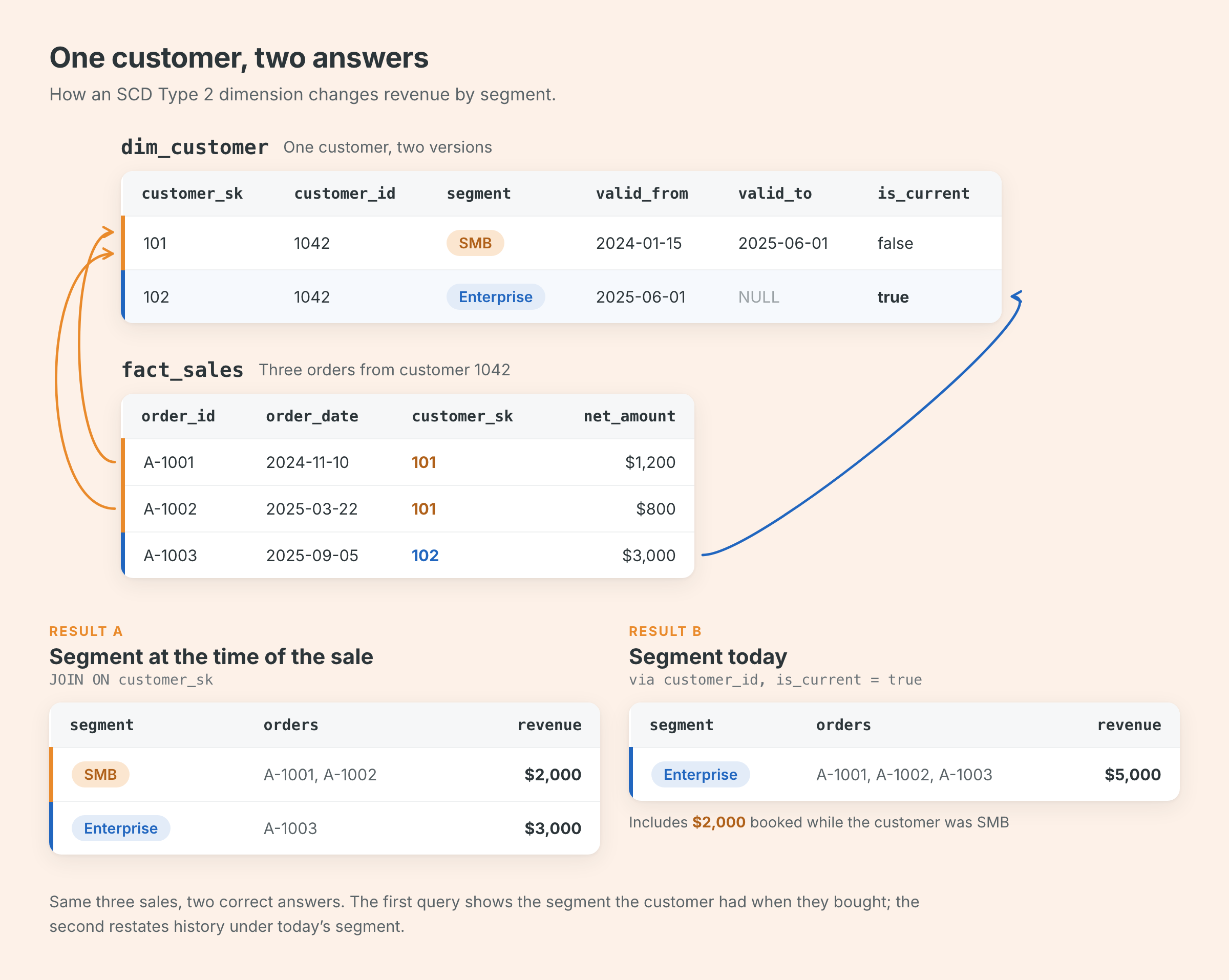
-- Segment at the time of the sale (point-in-time, thanks to SCD Type 2)
SELECT c.segment, SUM(f.net_amount) AS net_revenue
FROM gold.fact_sales f
JOIN gold.dim_customer c ON f.customer_sk = c.customer_sk
GROUP BY c.segment;

-- Segment today (re-stated with the current version of each customer)
SELECT cur.segment, SUM(f.net_amount) AS net_revenue
FROM gold.fact_sales f
JOIN gold.dim_customer c   ON f.customer_sk = c.customer_sk
JOIN gold.dim_customer cur ON c.customer_id = cur.customer_id AND cur.is_current
GROUP BY cur.segment;
That second pair is the reason SCD Type 2 exists. When a customer upgrades from SMB to Enterprise, their past purchases stay attributed to SMB in the first query, and the business can still restate everything under the current segment when needed. Both answers are correct; they answer different questions. The model makes the difference explicit instead of leaving it to whoever writes the query.
Making the Gold layer Genie-ready
Because the Gold layer is a clean Star Schema, connecting it to a Genie space is straightforward: add only the four Gold tables, and nothing from Bronze or Silver. For declaring the relationships between them (foreign keys, joins, and cardinality), see Hubert Dudek's guide on defining table relationships in Genie. Here we focus on what is specific to a dimensional model:
The pipeline already documents the model. The table comments declared in SDP (grain, SCD type, the definition of net_amount) are published to Unity Catalog and give Genie context with no extra work.
Teach Genie the SCD Type 2 semantics. A Genie space does not know that dim_customer has one row per version. State it as an instruction: "Join customers through customer_sk to get their attributes at the time of the sale. If the user asks for current values, join dim_customer again on customer_id with is_current = true." Add both segment queries above as example SQL, so Genie learns the difference between "then" and "now".
Pin down time semantics. While testing, Genie read "last quarter" as the current, still-incomplete quarter in one conversation and as the previous one in another. An explicit instruction, "last quarter always means the previous complete calendar quarter, never the current one", together with an example query that uses date_trunc('QUARTER', current_date()), made the answers consistent.
The instructions above teach Genie this specific model. For the governed, company-wide definitions that Genie Ontology adds on top, see Part 1 for the concepts and Part 2 for a hands-on walkthrough.
With that in place, a business user can ask "What was net revenue from Enterprise customers in Spain last quarter, by channel?" and get an answer grounded in the same definitions that power the official dashboards.
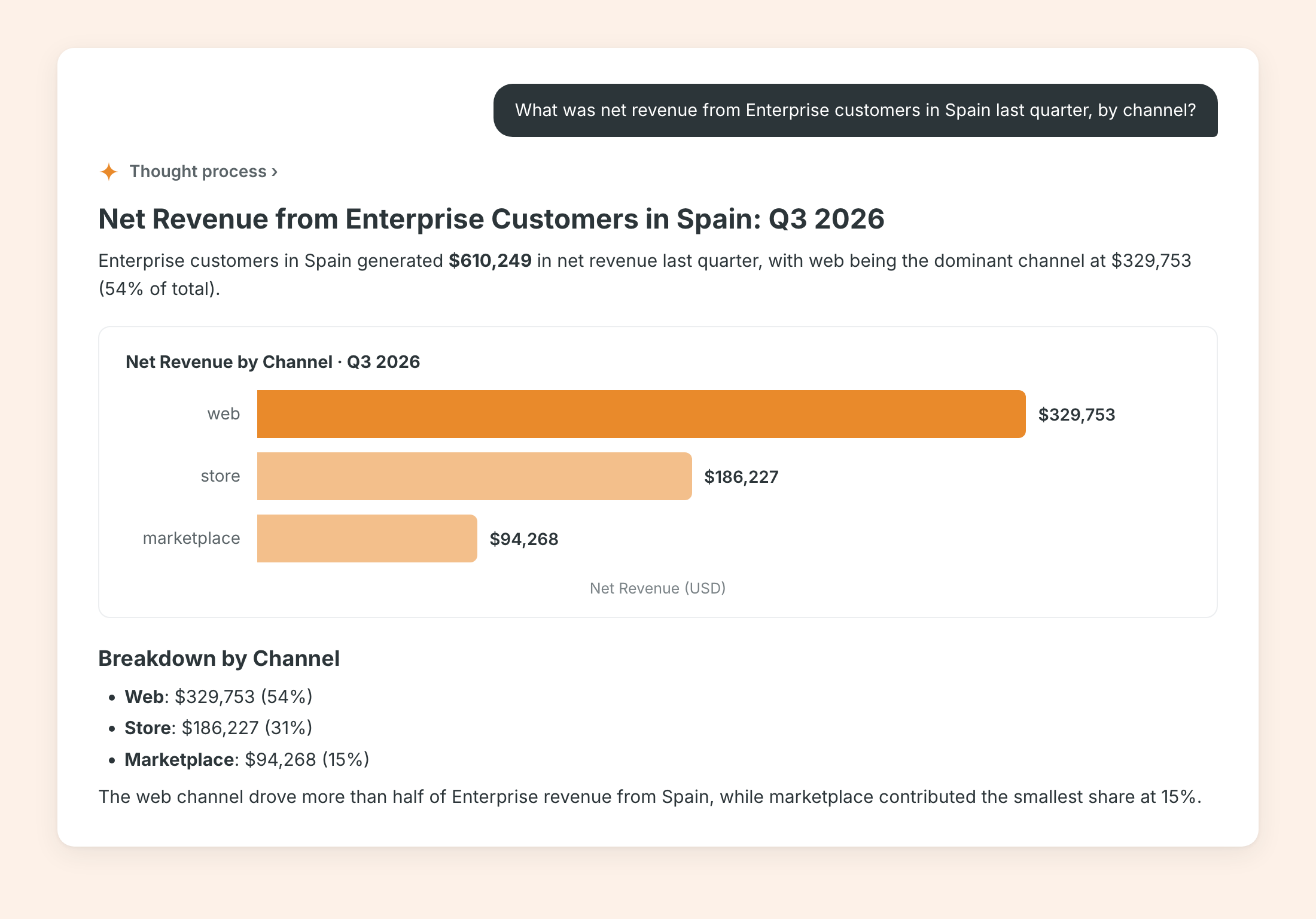
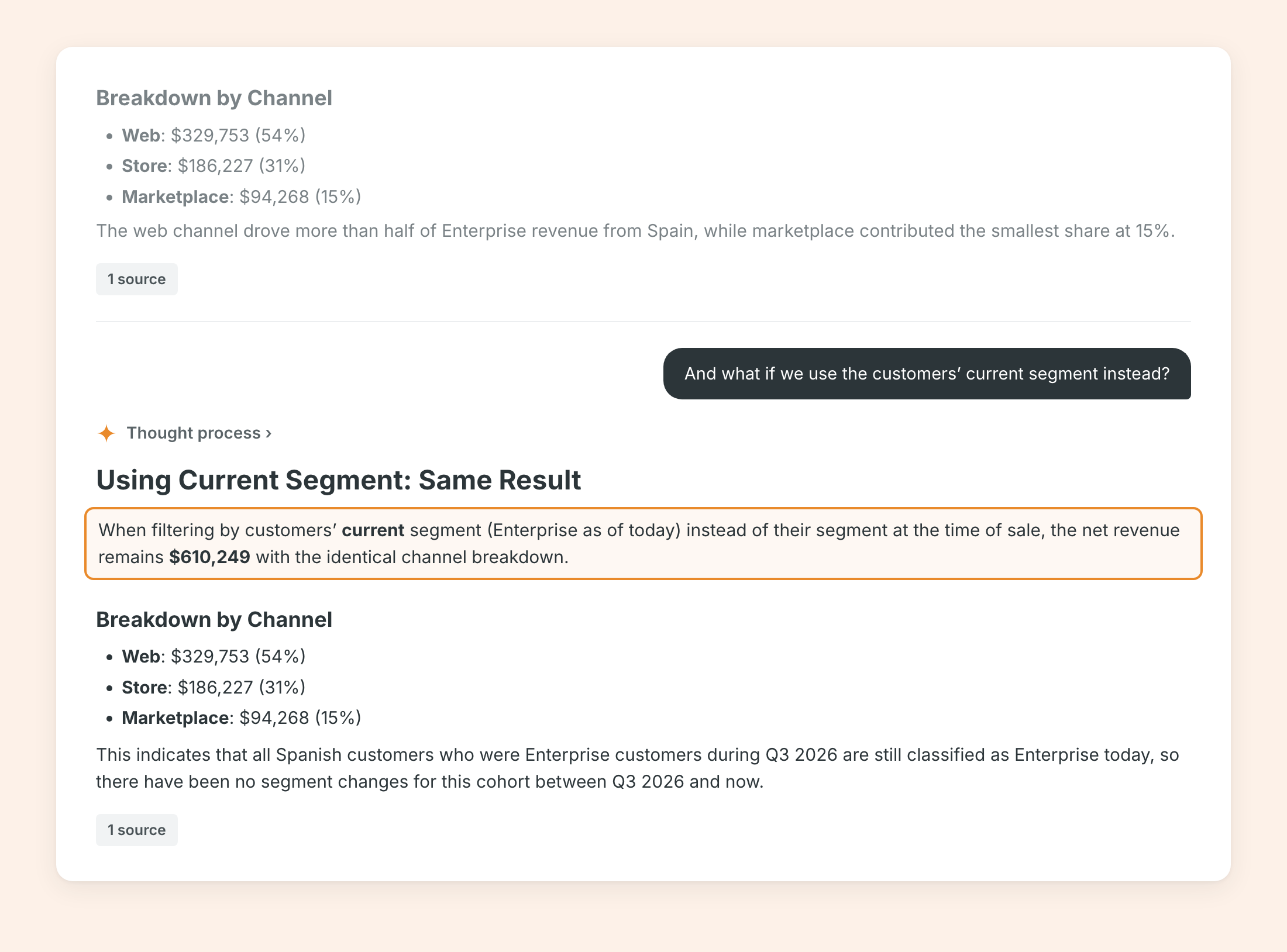
Genie answering a natural-language question over the Gold Star Schema.
Why combine dimensional modeling with SDP
Each technique is valuable alone. Together they reinforce each other:
Maintainable, declarative pipelines. Each table is a function that describes what the table is. No orchestration code, no hand-written MERGEand no checkpoint management. New engineers read the pipeline and understand the model.
Consistent business definitions. The grain, net_amount, the SCD strategy per dimension, and the data quality rules are declared once, in code, and versioned. Every dashboard and every Genie answer inherits them.
Incremental processing and automated change tracking. Streaming tables process only new data, materialized views refresh incrementally, and AUTO CDC maintains dimension history, including out-of-order events.
Reusable, business-ready datasets. The Gold layer is not built for one report. It is a shared analytical foundation for BI, ad hoc SQL, and AI-powered analytics alike.
What Comes Next
The model we built is a foundation, not a ceiling. Natural next steps include:
More facts on conformed dimensions, such as returns or inventory, reusing dim_customer, dim_product, and dim_date.
Unity Catalog metric views to define measures like net revenue once for BI and Genie. Part 2 of our Genie Ontology series shows how to build and certify one.
Quarantine tables for records dropped by expectations, so source owners can fix them.
The Model Is the Contract
Dimensional modeling has outlived every prediction of its death because it solves a problem technology alone does not: getting an organization to agree on what its data means.
Spark Declarative Pipelines remove most of the engineering friction it used to require. Dependencies are inferred, not orchestrated. History is declared, not merged. Quality is enforced in the table definition, not in a separate job. Incremental processing is the default, not an optimization.
What remains is what always mattered most: choosing the grain, deciding how each dimension should change, and defining each metric once.
Get the model right, declare it, and let the pipeline keep it right.