The Nightmare of Initial Load (And How to Tame It)

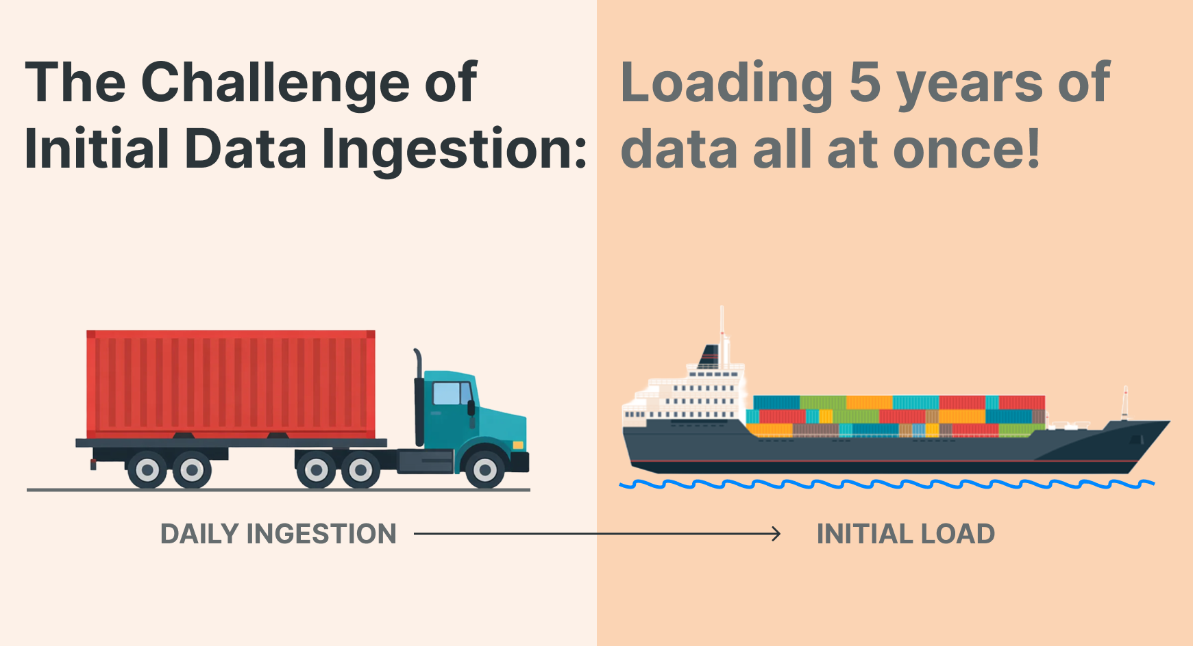
Initial loads can be a total nightmare. Imagine that every day you ingest 1 TB of data, but for the initial load, you need to ingest the last 5 years in a single pass. Roughly, that’s 1 TB × 365 days × 5 years = 1825 TB of data. Yikes!

This scenario is especially problematic for analytics event data (think, clickstream logs from Adobe or Google Analytics), where data accumulates over years, and every event matters for long-term trend analysis.

So how do you load years of historical data without bringing your data platform to its knees?

The Problem: One Pipeline, Two Very Different Jobs

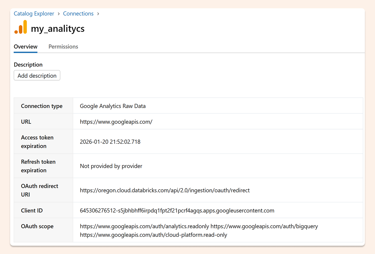
We have an excellent Lakeflow Connect integration for Google Analytics. After configuring Google Analytics to export to BigQuery and registering a connection in Unity Catalog, it's straightforward to define an ingestion pipeline.

Here's a basic pipeline definition using Databricks Asset Bundles (a declarative way to define data infrastructure as code):

resources:
  pipelines:
    pipeline_google_analytics_pipeline:
      name: google_analytics_pipeline
      ingestion_definition:
        connection_name: my_analityc
        objects:
          - table:
              source_catalog: analityc-484919
              source_schema: analytics_520647590
              source_table: events
              destination_catalog: ${var.catalog}
              destination_schema: ${var.schema}
        source_type: GA4_RAW_DATA

This works great for ongoing incremental loads. But try to ingest five years of historical events through this same pipeline, and it can take forever.

The root issue: incremental streaming and massive one-time backfills are fundamentally different workloads, and treating them the same creates operational headaches.

The Solution: Split Historical and Current Data

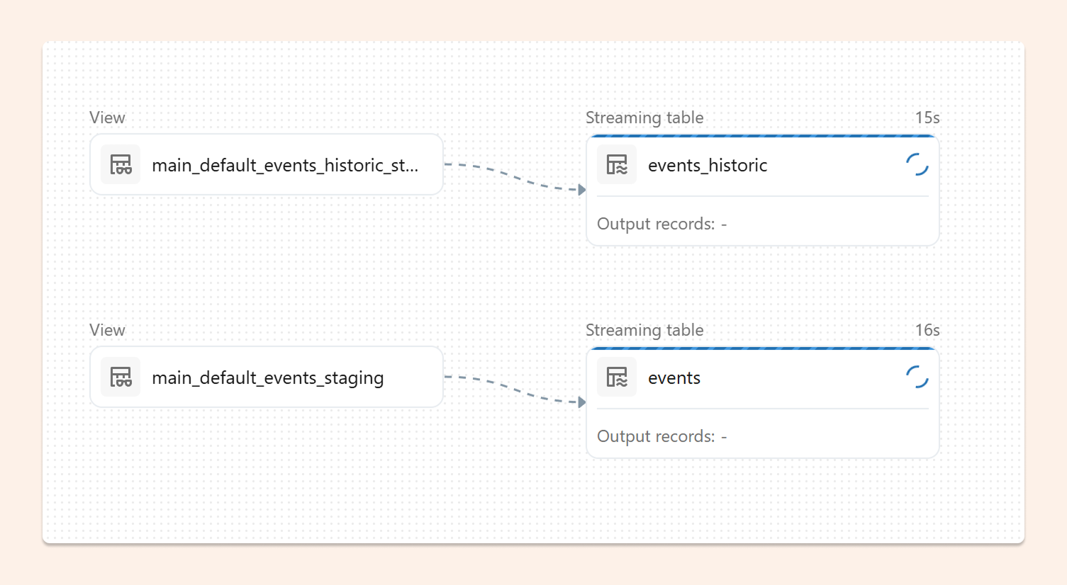
The best approach I've found is to use two separate Bronze tables: one for current events and one for historical events.

Why does this work?

1. Independent checkpoints: Each streaming table maintains its own checkpoint. If something goes wrong with the historical load, you can restart or refresh just that table without affecting your current data pipeline.

2. Resource isolation: You can tune compute resources differently for each workload—more aggressive parallelism for the one-time historical load, more conservative settings for ongoing incremental updates.

3. Clear operational boundaries: It's immediately obvious which pipeline handles which time period, making troubleshooting and monitoring much simpler.

The key technique is using a row filter in the table configuration to partition data by timestamp:

resources:
  pipelines:
    pipeline_google_analytics_pipeline:
      name: google_analytics_pipeline
      ingestion_definition:
        connection_name: my_analityc
        source_type: GA4_RAW_DATA
        objects:
          - table:
              source_catalog: analityc-484919
              source_schema: analytics_520647590
              source_table: events
              destination_catalog: ${var.catalog}
              destination_schema: ${var.schema}
              destination_table: events
              table_configuration:
                row_filter: "event_timestamp > '1768867200000000'"
          - table:
              source_catalog: analityc-484919
              source_schema: analytics_520647590
              source_table: events
              destination_catalog: ${var.catalog}
              destination_schema: ${var.schema}
              destination_table: events_historic
              table_configuration:
                row_filter: "event_timestamp =< '1768867200000000'"

Pro tip: For very large datasets (like multi-year web event logs), you could even create one Bronze table per year. The principle is the same—isolate workloads to prevent one failed load from cascading into others.

In practice, I'd create two separate pipelines (one for historic, one for current) and generate them programmatically using pyDabs to keep things DRY. For simplicity, the example above combines both into one pipeline definition.

Merging Back Together in Silver

Once you have two Bronze tables, the final step is combining them into a unified Silver table for downstream consumption.

In Databricks declarative pipelines, a Flow handles this perfectly. Flows can read from multiple sources and write to a single Delta table without concurrency conflicts.

Here's the elegant part: you can use INSERT INTO ONCE for the historical backfill—it runs exactly once and then stops—while the current events flow continuously streams new data.

CREATE OR REFRESH STREAMING TABLE silver_events;

CREATE FLOW silver_events_current AS
INSERT INTO silver_events BY NAME
SELECT * FROM stream(events);

CREATE FLOW silver_events_historical AS
INSERT INTO ONCE silver_events BY NAME
SELECT * FROM events_historic;

In this setup:

• silver_events_current continuously streams new events as they arrive

• silver_events_historical runs once to backfill old events, then stops

When to use continuous for both? If you expect late-arriving historical data (for example, if the source system could send belated backlog), run both flows as streaming by removing the ONCE keyword:

CREATE OR REFRESH STREAMING TABLE silver_events;

CREATE FLOW silver_events_current AS
INSERT INTO silver_events BY NAME
SELECT * FROM stream(events);

CREATE FLOW silver_events_historical AS
INSERT INTO silver_events BY NAME
SELECT * FROM stream(events_historic);

Both flows will now continuously sync their respective sources into the Silver table.

Making It Production-Ready

There are other ways to handle massive initial loads—for example, manually adjusting the row_filter cutoff and redeploying multiple times for different date ranges. But these ad-hoc approaches are harder to manage and make clean production deployments difficult.

My recommendation: Make the row_filter date a configurable variable with a sensible default (like the most recent January 1st). This gives you flexibility to control how much historical data to pull during initial load, without hard-coding dates in your pipelines.

For example:

variables:
  historical_cutoff_timestamp:
    default: "1704067200000000"  # Jan 1, 2024
    description: "Timestamp separating historical from current data"

# Then reference it in your row filters
table_configuration:
  row_filter: "event_timestamp > '${var.historical_cutoff_timestamp}'"

This approach works well with CI/CD pipelines—you can override the variable during deployment based on your environment or specific backfill needs.

The Bottom Line

Initial loads don't have to be nightmares. The key insight is recognizing that massive one-time backfills and incremental streaming are different workloads that deserve different treatment.

By splitting them into separate Bronze tables with independent checkpoints, you gain:

• Operational resilience: Failures in one pipeline don't cascade

• Resource optimization: Tune each workload independently

• Clearer troubleshooting: Separate concerns make debugging simpler

And with Flows in Silver, you can merge everything back together cleanly—using INSERT INTO ONCE for the historical backfill and continuous streaming for current events.

The result? A production-ready pattern that handles both the initial tsunami of historical data and the steady stream of ongoing events without breaking a sweat.